What is Image Classification?
Image classification refers to the process of assigning classes to individual pixels within remotely sensed images. There are two main methods of classification: supervised and unsupervised.
Supervised classification: You define the relevant classes and train the system using samples for each class. The system learns from these samples and uses them to classify the entire image.
Unsupervised classification: The system groups pixels with similar spectral characteristics into classes without predefined categories. This can be useful for exploring large datasets without prior knowledge of categories.
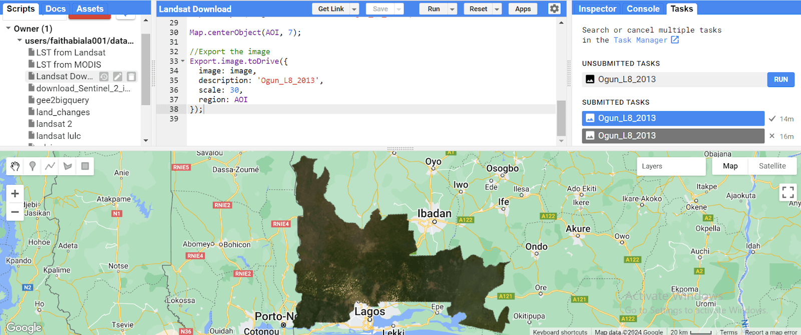
This tutorial guides you through performing supervised image classification using Landsat 8 imagery in ArcGIS Pro. To learn how to download Landsat imagery, check here.
Pro Tip: You can download only the specific bands you need for the classification.
Let's get started!
Step 1: Adding Data to ArcGIS Pro
Common Landsat 8 band combinations for image classification include:
(4, 3, 2) - Natural/True Color
(5, 4, 3) - Color Infrared (Vegetation)
(7, 6, 4) - False Color (Urban)
For more information on band combinations, refer to the Additional Resources.
To begin:
Open a new ArcGIS Pro project.
In the Map tab, add your data.

For this tutorial, I'll be using bands (5, 4, 3). Navigate to your data location and add bands 3, 4, and 5.

Step 2: Creating a Band Composite
We'll now combine the three bands into one composite image.
Go to the Analysis tab and click on Tools. This opens the Geoprocessing Toolbox.

In the toolbox search bar, type "Composite Bands" and select it.
Add bands 3, 4, and 5 to the "Input Raster" section.
Set the "Output Raster" to your desired location and filename. (Pro Tip: Always include ".tif" in your chosen name when dealing with raster.)
Click "Run." Once completed, the composite image will be added to your map frame.


Step 3: Clip to Your Area of Interest (AOI)
There are two ways to clip your data to your desired area of interest (AOI):
Using the "Clip Raster" Tool:
In the Geoprocessing Toolbox search bar, type "Clip Raster" and select it.
Set the "Input Raster" to the output of the composite band process.
Set the "Output Extent" to your AOI shapefile or polygon feature.
Set the "Output Raster Dataset" to your desired output name and location (remember to include ".tif").
Check the box "Use Input Features for Clipping Geometry."
Ensure the "NoData Value" is set to 0.
Click "Run."

Using the "Extract by Mask" Tool:
In the search bar, type "Extract by Mask" and select it.
Set the "Input raster" to the composite band output.
Set the "Input raster or feature mask data" to your AOI shapefile or polygon feature.
Set your desired output name and location in the "Output raster" field.
Make sure "Extraction Area" is set to "Inside" and click "Run."

Step 4: Training Samples for Image Classification
With our area of interest (AOI) defined, let's train samples for image classification:
In the Imagery tab, go to Classification Tools and select “Training Samples Manager.”

Create a new schema:

Right-click "New Schema," choose "Edit Properties," set a desired name, and click "Save."

Right-click your schema and click on “Add New Class” to add new classes based on your study area (in this tutorial, "Waterbody," "Bareland," "Built-Up," "Vegetation," which is based on the Land Use classes present in my AOI). Repeat for each class.

Train samples for each class:
Select a class (e.g., "Waterbody").

Choose a tool (rectangle, circle, or polygon) for sketching samples. The cursor will turn into a plus symbol.
Sketch your training samples by clicking and dragging your chosen shape.
Collapse the samples in the Training Sample Manager after sketching.

Repeat for all classes until your samples resemble the image below.

Save your trained samples to your desired location.
Step 5: Image Classification
With our trained samples ready, let's perform image classification.
In the Imagery tab, go to “Classification Tools” and select "Classify”
Set the "Classifier" to "Maximum Likelihood".
Input your trained samples in the "Training Samples" bar.
Set the "Output Classified Dataset" to your desired name and location.
Click "Run".

Voila! You should now have a classified image. Style it using appropriate map symbols and styling for clarity.
The image below represents the classified Land Use classes of Osogbo Zone: Waterbody, Bareland, Built-Up, and Vegetation.

Additional Resources:
Image Classification Documentation
Band Combinations for Landsat 8